


- Introduction
- Section 1: Background
- Section 2: Error Budgets with Lidar
- Section 3: How to Test Accuracy with Lidar
- Section 4: DJI L1 Absolute and Relative Accuracy Assessments
- Section 5: Project Level Testing
- Testing Conclusions
- References
The debut of the DJI L1 lidar system to the aerial surveying market brought with it the idea that equipment such as this could be affordable and offered at a lower price point compared to what has been seen historically. The DJI L1 lidar system costs a fraction of the price compared to its competitors’ products so it is normal to question the quality of the product. If a retailer offered you an alternative to an iPhone for $30 but swore that it was just as good as an iPhone, would you believe them?
The affordability of the DJI L1 lidar system has raised a few eyebrows but as technology has advanced, prices have decreased. For example, the Compaq Portable computer was selling for more than $8,000 dollars in 1987. Today, you can find “portable computers” aka laptops, for under $200. Is the DJI L1 lidar system a sign of advancements in technology making digital products more accessible? Or is it too good to be true? Our team at Alynix dedicated a year to researching the DJI L1 and its accuracies by gathering data from both individual and long-term projects. We are here today telling you what we found.

-

Zenmuse L1
$8,543.00 – $9,326.00 Select options This product has multiple variants. The options may be chosen on the product page
Before we advance any further, while many are already familiar with these concepts, some of you may not be. If you are already familiar with these concepts, feel free to advance to Section 2.
Let us start with the word “lidar” and how to even say it. First, it is pronounced laɪdɑːr or lie-dar. It is an acronym meaning Light Detecting and Ranging. That still may mean nothing to you so let us talk about concepts that are familiar to you: sonar and radar.
You have heard of those in science or history class during high school and those are acronyms as well. Sonar means Sound Navigation and Ranging, and the acronym radar means Radio Detecting and Ranging. Are we seeing a pattern here yet? There is a pattern because the technologies act in a comparable way but vary in the type of energy that is used to complete the process. Lidar, sonar, and radar all can be used to measure distance and are all ranging devices. They work by sending out a pulse of energy to an object so that the energy can bounce off the object and return to the system of origin, bringing with it a distance measurement. Sonar was created in 1918, followed by radar in 1935 and lidar in 1961.
Now we know that lidar means Light Detecting and Ranging but how exactly does it work? The first step is knowing the starting point. Lidar is used for measuring ranges so there need to be at least two clear points between which distance can be measured. Lidar cannot see through trees despite what many believe.
There are different lidar technologies available today that use different approaches. Today we will be discussing the lidar technology used by most mapping systems called “time-of-flight.” To further break that down, we will be talking about time-of-flight systems that are on a moving vehicle. We refer to these as “kinematic” systems. To understand how a kinematic time-of-flight lidar system works, we need to understand the three major components, the lidar, IMU, and GNSS.
The first component to understand is the lidar itself. Lidar produces “pulses” of light. A lidar system can modulate how many pulses of light it sends out and how fast. Those pulses of light travel at the speed of light to hit an object and then bounce back to the detector.
You can think of it as a race. When you send a pulse of light, you start a stopwatch. That pulse of light races from the sensor to the object you want to measure and back to the detector. When the pulse of light makes it back, you stop the timer. With some basic physics we can use this time measurement to get a distance. The speed of light is a constant. We know how fast the light was going. It ran the race at 300,000 km/second! We can take the speed it traveled and multiply it by the time it took and now we know how long it took to get there and back again. The last thing we need to do is cut the distance in half to understand how far away it was to the end.


Getting a distance from one place to another place is great but it does not tell us much if we do not know where we are. With a stationary LiDAR, we can measure the location of the sensor so that we have a starting point. This is great if we are not moving but what if we want to measure from a moving object like a car, drone, or airplane? To do this, we need to know where we are in space while moving. To do this, we use global navigation satellite systems or GNSS. GNSS is something that anyone with a smartphone has access to. In space, there are several constellations of satellites. These satellites broadcast precise orbit information and time stamps. Our phones can read this information and triangulate from a minimum of three satellites its position on the earth. Your phone can determine where you are with an accuracy of about ten meters. The equipment we use with lidar can determine our position up to about 3 cm!
Next, the lidar needs to understand its orientation (also known as direction or bearing) to give an accurate measurement. With a static scanner, bearing can be established using conventional survey methods and then using mechanical means to establish orientation.
When systems are moving, or “kinematic,” we need a way to understand our orientation while moving. The most common way of doing this is utilizing an inertial measurement unit or IMU. This is an electronic device that can report information such as orientation or acceleration. There are several types of IMUs that vary in cost and accuracy. Traditionally, IMUs had spinning parts and were expensive to produce. Most IMUs today are referred to as microelectronic mechanical systems or MEMS and are less expensive to produce.

Other orientation methods
There are two other methods for determining orientation (and positioning) and they are called slam and optical flow. Slam is yet another acronym and it mean simultaneous localization and mapping. It is a broad group of methods that use remotely sensed data to determine your positioning.
Optical flow is slightly different in that it uses the apparent motion of objects caused by the motion of the camera to help determine positioning. Optical flow is only locally consistent, meaning it is incrementally estimating a path vs. trying to obtain a globally consistent estimate of the orientation. This can be extremely complicated, but it is important when understanding the L1 and positional errors. The DJI L1 uses an optical flow sensor to help optimize the orientation or overall pose.

So now you have the three main components of how lidar functions: the position in space (GNSS), its orientation (IMU and Optical Flow), and the laser ranging and detecting. There is one more key component to lidar. The component that brings all these elements together precisely is time. Very precise time. We need a way to synchronize all these elements. Lidar units have a timing board that is used to synchronize everything together and that is synchronized using GPS time.
You may be wondering why lidar even matters to you. Lidar is an efficient tool to measure the 3D world. Lidar allows us to create dense point clouds of heavily forested areas so that we can understand the biomass or the topography underneath the canopy. It can be used to map the as-built world such as roads, utility lines, or landfills. By doing this from a distance or “remotely sensed” we can measure, map, and model large areas quickly and cost effectively.
So, what does all this background have to do with the L1’s accuracy potential? All these elements play a role in a systems overall error budget. The error budget is the acceptable accuracy of the project minus the total combination of all these elements. This can vary tremendously depend on the project type and use case or “intended mapping purposes.” Some projects require an extremely high precision and accuracy while others do not. For example, error budgets will be quite different if you are looking for 2-foot contours in a wooded area for raw land development vs. a topographical surface model to redesign a road. These have vastly different intended mapping purposes and require a different level of precision. As a result, each project will have quite different error budgets.
Although lidar can provide precise and accurate measurements, there are so many components that go into getting that measurements that if even just one of those is inaccurate, it will compound increasing the overall accuracy of the dataset. Therefore, it is important to understand the achievable accuracy and the level of precision of the components that make up our error budget. Detailed below are some of the errors that can occur when using lidar.

Let us look at some of the inherit accuracy errors of these components of a kinematic lidar system, specifically the L1. The first type of error can be vertical error, which can be determined using measurements from flat terrain. There will always be a margin of error, but with vertical error, the further the distance, the more the error increases.
For example, starting with the laser itself, the DJI L1 utilizes the Livox Avia scanner. The Avia scanner in laboratory settings has a precision of 2 cm (.78 inches) at 65 feet. On a linear scale, which means the sensor only has a precision of 4.9 inches when flown at 400 ft. The higher you go with the device, the greater the vertical error.

Five inches could make a significant difference depending on the project. For example, it may not seem like a lot when you’re trying to understand which way the water drains in an undeveloped forest, but if a road in Florida was all the sudden five inches taller, that would make a big difference to where the water goes so it’s important to understand your vertical error and what your tools can produce.

Next, we need to factor in the GNSS error. Again, there are a lot of elements that can affect this, and you can process the L1 in either RTK mode or in PPK mode. In general, your expected accuracy for your GNSS point will be within ¾ of an inch horizontally and about two inches vertically.

Then we have the IMU and the optical flow sensor. There is not any published information available on the optical flow sensor for the L1, but the IMU used in the L1 has an error of 0.03 degrees in both the pitch (the rotation around the side-to-side axis) and roll (the rotation around the front-to-back axis) direction. The IMU has an error of 0.08 degrees in the yaw (rotation around the vertical axis) direction. It is common for the yaw direction to be worse than the roll and pitch direction.
DJI L1 sources of Error | |||||
| Altitude (ft) | Laser accuracy (inches) | GPS Elevation accuracy (inches) | GPS Horizontal accuracy (inches) | IMU Horizontal Accuracy (inches) | Total Potential Error Propagation (inches) |
| 100 ft | 1.2 | 2.0 | 0.8 | 0.62 – 1.67 | 4.62 – 5.67 |
| 200ft | 2.4 | 2.0 | 0.8 | 1.25 – 3.35 | 6.45 – 8.55 |
| 400ft | 4.9 | 2.0 | 0.8 | 2.5 – 6.70 | 10.2 – 14.4 |
As you can see from the table above, as the altitude increases, most of the error margins increase as well (except for those associated with GPS. The error rates that you have been presented are those that have been calculated in laboratory settings or by the manufacturer itself. We can use this data about the errors, but we must also ensure that we are assessing the accuracy of the products that are used with the laser. There needs to a clear and replicable testing process to see how the product truly works, which is what we conducted and will be discussed in the testing section.
There are several entities that have developed accuracy standards for geographical data. This started as far back as 1941 when The Bureau of the Budget in conjunction with the American Society of Photogrammetry and Remote Sensing (ASPRS) developed the National Map Accuracy Standards (NMAS). Since this time, there have been several different standards that have been developed. Given the advancements in technology, specifically for modern data collection, the standards for geographical data have changed as well.

The new American Society for Photogrammetry and Remote Sensing’s (ASPRS) standard is called the ASPRS Positional Accuracy Standards for Digital Geospatial Data. The most recent version is Edition 1 version 1.0 from November of 2014. These standards are intended to be agnostic to best practices or methodologies used to collect data. They focus on the positional accuracy of final geospatial products. This specification covers quite a few topics but for our purposes today, we are going to focus on assessing our absolute and relative vertical accuracy.
Absolute accuracy is one that accounts for all the systematic and random errors. It also relates the modeled elevation to the true elevation with respect to an established vertical data point that has been geo-referenced. This means that we can go to the same location in the real-world time after time and achieve the same measurement and that measurement agrees with other methodologies in respect to that coordinate system.

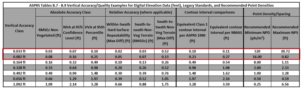
The Graphs shown here are tables B7, B8, and B9 from the ASPRS specification. There is a lot here to understand but we are going to simplify into common surveyor terms. We will go through each of these assessments to determine the tested accuracy of the DJI L1 over multiple projects and flights.
Before we start our accuracy assessment, we need to define two desired vertical accuracies. For ease of use, we will call them “standard grade” and “max grade.” These are entirely arbitrary but will help us understand the achievable accuracies of the DJI L1.
Standard Grade
Let us say we were doing a survey for the planning of a project for raw land development. We may want to produce a surface suitable for 1-foot contours (see the red box on the graph below). For that, we want our tested vertical accuracy to be better than three tenths of a foot RMSEz for hard shots and better than one foot for vegetated topo shots (VVA). We want our swath-to-swath accuracy on hard surfaces to be less than 0.2 ft and a point density greater than two points per square meter. For most of the mapping in the US, this is the “standard grade” required.

Max Grade
Imagine we are producing a map for a new road development project. For that, we would want our tested vertical accuracy to be better than six hundredths of a foot (see the red box on the graph) on hard surfaces. This is somewhere between the two highest vertical accuracy classes and is achieved today utilizing conventional survey approaches (total stations and digital leveling) and mobile lidar. For this accuracy, we want our RMSE to be better than 0.06 ft in non-vegetated areas and our VVA to be better than 0.18 ft. Our swath-to-swath accuracy needs to be no greater than 0.035 ft.
According to section 7.9 of the ASRPS positional accuracy standards, the checkpoint accuracy must be three times greater than the required accuracy of the data. So, for “standard grade,” we need our checkpoints to be at least 0.10 ft vertical accuracy to assess data to a 0.30 ft. RMSEz. This can be achieved with conventional GPS equipment which typically has a horizontal accuracy of about 0.06 ft. horizontally and about 0.10 ft. vertically.
If we are trying to assess our data to the “max grade,” GPS alone will not do; we need to achieve an accuracy of 0.02 ft. or better. That is a quarter inch. These types of accuracies require conventional leveling to be achieved and thus require more equipment and technology. This also raises an interesting paradox. As we get closer to an accuracy of zero, the less accurately we can measure the accuracy of the data. The tools are no longer good enough and tiny changes in the earth day to day start to introduce error.
Relative accuracy measures the point-to-point accuracy within a specific dataset. The vertical difference between two points is measured and then compared to the difference in elevation to a reference dataset. There are two types of relative accuracy we are interested in testing on the L1. They are the laser head precision and swath-to-swath accuracy.

The noise spread in a point cloud shows its relative accuracy for each shot taken. This is commonly shown with a bullseye, as shown in the image below. If we are averaging around the center of the target but our spread is high, this means that the laser is accurate, but its precision is low. This is quite common with what we typically deem as “automotive grade” lasers. The L1 uses this type of laser which has a cheaper diode, but the tradeoff is that it has a lower precision. The same is true for quite a few drone lidar sensors. There are very few “mapping grade” (which are on the higher end) lasers, and they are more expensive.

So, what type of repeatability within-swath do we need for our two examples? If we want to produce “Standard grade,” our noise spread on flat surfaces should be less than ± 0.2 ft. For our “max grade,” we need to be better than ±0.0375 ft.

The second type of relative accuracy we need to consider is swath to swath. To collect lidar data for large projects, we need to take multiple passes for complete coverage. There is overlap between portions of the swaths to prevent data gaps or to ensure the required level of point density. A common way to visualize this is by creating swath separation images as shown below.

Going back to our two examples, for “standard grade,” our individual flight lines need to match each other within 0.26 ft on average with a maximum mismatch of 0.52 ft. (see the red boxes on the graph above). For “max grade,” we need that to be closer to 0.05 ft with a maximum mismatch of less than 0.0975 ft.

So now we have established the sources of error for our sensor, the different accuracy requirements to validate absolute accuracy and relative accuracy. Next, we need to design an experiment that allows us to assess all these components, specifically for the DJI L1 to understand the achievable accuracies.
Since products like the DJI L1 can be used in a multitude of contexts, we needed to assess it in several different settings. We wanted to see how well it could perform with a highly controlled test site to get detailed information in a single project (this is our micro testing). We also wanted to understand how the L1 can perform over time, through a large cross section of projects (this is our macro testing). It is quite possible to have a single project perform very well and then have some that do not, so it is important to use a variety of projects for validation.
First, let us start with the performance of the L1 over time. We have been utilizing DJI L1 with customers on controlled projects since November of 2021. In that time, we have flown a total of 34 DJI L1 projects that had the highest level of control set (total station or digitally leveled GPS control). For each of those projects, TerraSolid’s TerraScan L1 wizard was run for processing, and a vertical accuracy assessment was performed.

To perform this assessment, a TIN model of ground classified points is compared to the elevation of each validation point (a type of data that measures the distance from the surface to a known elevation).


Then, the delta of those two values is used to calculate the root mean square error (RMSEz), project minimum and maximum as well as the standard deviation. From here, a z debias is performed to bring the point cloud to the mean z error. This is a total block adjustment and is common in lidar processing.

If you look at the information in the red box of the chart below, of those projects, the average RMSEz was just under seven hundredths (0.067) of a foot. The minimum RMSE was 0.01 ft, and the worst project was 0.23 ft, which is still within the accuracy requirements for “standard grade” projects. Based on this one assessment, 100% of projects flown with precision ground control were suitable for “standard grade” and 40% had a vertical accuracy that meet the “max grade” requirements.

Next, all points were calculated together to get a total RMSE and standard deviation for all projects with leveled control. This was a total of 318 individual validation points over the course of a year. The total RMSEz (ft) for all 318 points was 0.082 feet and the standard deviation was the same. A histogram of all points was plotted to see the spread. There are some outliers, but it mostly follows a Gaussian curve.

While this is not a perfect sampling, it is it is statistically significant. These projects cover the course of an entire year over multiple states, in many projections and conditions. While this alone is not enough evidence to say definitively that the L1 can support “standard grade” mapping, it does show that you can consistently achieve absolute vertical accuracies suitable for “standard grade” mapping. In some cases, it was found to be suitable for “max grade” topo but as we mentioned before, this is not the only criteria we need to assess. We need to look at relative accuracy and test against a greater concentration of points over a single project. To do this we setup a more rigorous test site with a carefully controlled setting for our micro testing.

In December of 2021, we had the opportunity to setup a more rigorous experiment to assess the accuracy of the L1 sensor. George Butler and Associates (GBA) asked us to help participate in a study to assess the accuracy of several different systems and methodologies. GBA was awarded a survey contract through the Kansas Transit Authority to perform a “design grade” survey on a stretch of highway on I35 near Emporia Kansas. The site was a bridge section of the highway and one mile on each side of the highway leading up to the bridge. They survey was performed on the road leading up to the bridge and not the bridge itself due to potential errors from movement of the bridge.

The survey crew at GBA performed a complete topographical conventional survey of the site. This was performed in an unconventional way. For each topo shot that was taken, the field crew placed a dot with spray paint so that it could be located using multiple methods. GPS survey was performed using an onsite local network with Trimble R12i rover and base stations. Dual occupancies were performed to ensure a horizontal accuracy greater than 0.02 ft. Next, a Trimble DINI digital level was used to calculate the elevation of each shot to less than 0.02 ft. At the same time, aerial and mobile lidar control was set for the project site by placing a mag nail and spray painting a circle around the control point. Control was measured in using a robotic total station. A total of thirty ground control targets were set.

After the survey was completed, several technologies were used on site for comparison. All data was collected within a week of each other. To compare point clouds from a higher accuracy system, two mobile lidar systems were brought out and used to collect the site. The first system was the Trimble MX50, and the second system was the Trimble MX9. At the same time, manned aerial mapping was collected at 1000 ft AGL utilizing a Z/I DMCII 140 with a total megapixel count of 140 and aground sampling distance of 5 cm. Multiple flights using the DJI P1 were performed as well. For the purposes of this presentation, we will not be talking about any of the other sensor data collected. We will be focusing on the L1 and its comparison to the conventional data.
The DJI L1 was flown three times using different settings for comparison. Repetitive mode, which oscillated the lidar scan left and right of nadir was used for two missions at two altitudes and one mission using non-repetitive mode, oscillating the scanner left right, forwards, and backwards was used for the third mission. Our assumption going into these flights is that the repetitive mode would be less noisy and that the lower altitude flight would have a higher absolute accuracy.

Like the test performed on all previous projects, the same vertical accuracy assessment was performed on the DJI L1 for these three flights. We first compared the control points to the classified point cloud produced from the DJI L1 after classifying using TerraSolid’s L1 processing wizard.

As you can see, the fit for all three flights was quite good with the worst flight being the lowest altitude flight (flight 2) This is primarily due to checkpoint thirty which has a significant outlier that we will investigate shortly. Based on these results and our first vertical requirement in the ASPRS specification, all three flights are suitable for “standard grade: and 2 of the three projects are suitable for “max grade” topo.

Next, we wanted to look at more detailed information about the flight. The thirty control points are statistically significant and are very accurate but what about all the leveled survey shots? To check that, we ran the same process on each shot that was taken in the roadway. This totaled 176 unique shots.

For the tested leveled survey shots of all three flights, our greatest outlier for all three flights was -0.263 ft. Our RMSEz for each project was 0.05 ft. or below which are phenomenal results when comparing all hard shots that are digitally leveled.
From these results, you can conclude that there is a strong correlated fit between the two datasets and based on this measured metric alone, the DJI L1 is suitable for producing both “standard grade” mapping and “max grade” topo. This, however, is only one of our assessments we need to perform. We need to also understand the relative accuracy of the L1. To do that, we need to assess its point-to-point accuracy and swath to swath accuracy.

Now that we know the absolute accuracy fit of the DJI L1, we need to look at the relative fit or noise spread in the point cloud. If you were to open an L1 point cloud and draw profile lines of the point cloud. The first thing you might observe is that it looks noisy. In fact, if you measure the distribution of that profile line. You might find it to be as large as 0.5 ft. So, the question becomes. If my point cloud has a relative accuracy as large as 0.5 ft, how are you measuring absolute accuracies that are as low as 0.03 ft? Our planar fitting analysis will try to answer this question. Its important to mention that all testing was completed using older versions of DJI Terra. Version 3.6 has a new smoothing algorithm to reduce this type of noise. We have not evaluated that algorithm yet.

To understand how our assessed absolute accuracy can so high, we need to understand our point-to-point relative accuracy. To do that, we needed to understand the distribution of the points over a planar surface. Because our datasets were over a flat road, we have a very planar feature to run our assessment with.
To evaluate our data, we broke the three datasets into two groups. The first group was all unclassified points. This is to understand the fit of the raw point cloud from the DJI L1 system. For the second group, we ran Terrasolid’s TerraScan L1 classification wizard to separate estimated ground points from the rest of the points. In point cloud processing, we often separate our ground classified points from the rest of our points for surface creation. Terrasolid has created a macro that custom built to the DJI L1 that simplifies this process down to a few parameters.

While a road is planar, it does have undulation. To minimize the effect of this, we broke each mission into fifty-three unique tiles over the surface of the road. We needed to limit the size to planar areas due to the slow elevation gain and rutting of the road. Each tile was the width of the highway road surface and 50 ft long.

The data in each tile are arrays of 3D vectors denoting a location in xyz-space. By assuming that each tile has a 2D plane that can be fit in a 3D space, we are able to calculate a best fit plane to each tile. Now we can calculate how well the point cloud matches the plane above and below for each tile. Next, we can consolidate the results of all those planes for the length of the road.
Below is an example of one of those planar models run on the exact same tile. The first image shows all points from the raw point cloud and the second image showed the ground classified points created by Terrasolid. The first image is noisy making it difficult to decern where the road is. The second image shows you some of the road features where the road becomes nonplanar.

The points from each plane were displayed in a histogram for visualization. By looking at the histogram of both planes, you can see that the distribution of the unclassified points are fairly concentrated around the mean but the min max is much higher at nearly 0.2 ft in each direction. This is similar to what we measured in our profile views earlier. The ground classified points on the other hand have a much more Gausian distribution and have a much lower min max distrubtion. They have a min max spead of about 0.04 ft. This represents a 5x improvement!

When we look at the consolidated histograms for all six datasets, we start to see a pattern emerge between the classified and unclassified data.

Now that we have a planar fit model for these datasets, we can go back to our ASPRS specifications for planar fit and compare the two. Our first scenario for “standard grade” requires us to have a within-swath max difference better than 0.2 ft. Based on these criteria and how the test was conducted, we had point outliers that went above that for all flights with the exception for the ground classified points for flight one. Its important to note that the unclassified point clouds did include some vehicles and points inside of drain grates that have skewed the results.

What is interesting is that at 95%, all our flights perform quite a bit better than that. At the 95% all ground classified datasets were suitable for “standard grade” mapping and remarkably close for “max grade” mapping. Its also important to point out that our approach is a more rigorous approach than what is recommended. ASPRS recommends performing this test using rasterized datasets that are twice the nominal point spacing. Utilizing this approach, many of the statistical outliers in our dataset would be lost.

When it comes to “automotive grade” lasers, there is no question that their precision is quite a bit lower than “topographical” mapping lasers. What is interesting about this planar analysis is our ability to clean that noise up considerably using algorithms such as the TerraSolid wizard. When it comes to this test, it is worth reviewing and clarifying how this test is performed by ASPRS. If we can create a derivative product that meets the within-swath precision required, should that be acceptable?
The last criteria we need to investigate is how well each swath or flightline aligns to each other. Our planar model earlier is a good indicator of the fit within a flightline to show the precision of the laser itself but swath to swath helps us understand how well the different flight lines align to each other. This helps us understand our inertial navigation system (INS) accuracies a little better. As we saw earlier, our IMU and GPS inaccuracies have the potential to be quite high however DJI utilizes optical flow to help compensate for some errors.

To assess the swath to swath fit, we used both a quantitative and qualitative approach. For the quantitative approach, each swath or flight line was separated out by plane segment. Using a similar approach to the planar fit test. A 3D plane was fit to the mean of all flights per segment. Next, we compared each flight line to the mean plane to determine the offset. This was only performed on the planar sections of the mission and does not represent a complete swath to swath analysis.

The results were fairly simillar to the planar fitting test. For the unclassified points flights we observed a larger deviation which is expected and the ground classified flights had a tigher fit with a deviation that was about half that of the unclassified points.

The qualitative test is an assesment of all overlaping points swath to swath. This is comonly refered to as a delta z raster. Its performed by creating a rasterized image that calculates the max distance for a pixel between swaths. The raster cell size should be at least 2 times the nominal point spacing of the lidar. Our nps is about 0.3 ft. which is adequate for our chosen pixel size (1 ft.).

Visually we can see that the swath-to-swath fit is good for all three flights. We do not see any spots where the GPS has drifted or boresight issues which would be indicated by yellow or red colors towards the edge of a swath or near a steep bank like the one near the bridge.
While our Delta Z raster approach is not a quantitative approach, it is a straightforward way to visually interpret the swath to swath fit. Based on this assessment, the swath to swath fit for each flight is quite high and suitable for “standard grade” mapping and quite possibly for “max grade” as well however, its difficult to definitively know using this approach. Its important to remember that this test is to verify the quality of the INS system which includes the GPS, IMU, and the optical flow sensor for the L1. The further you get away from your target, the greater our IMU errors will be. All three flights were performed at 200 ft or below and do not assess the maximum distance that can be legally flown in the United States.
The final test we will conduct is very straightforward. We need to verify our point density or conversely our point spacing. For all three missions, we flew at an average point density of four hundred points per square meter which is much higher than required however, our filtering reduces that down quite a bit to just the points we need to represent the ground surface. Based on our specification from ASPRS, we need a point density greater than twenty points per square meter and a nominal point spacing of less than 0.72 ft for “max grade” mapping. Our thinning process gave us a ground point density of twenty-five points per square meter for each mission and a nominal point spacing of 0.3 ft. for our classified ground points.


While there is additional testing, we would like to do such as comparison to the mobile lidar and aerial lidar collections, we hope that we have presented some evidence to inform you about the pros and cons of using the DJI L1 for topographical mapping. We believe that the DJI L1 is more than acceptable to produce “standard grade” based on the ASPRS specification however it is not perfect. One of the main things that someone needs to consider when using the DJI L1 or any automotive grade sensor is the precision of the laser itself. Without the proper ground filtering such as the one provided in TerraSolid, the precision of the system is quite low and not suitable for “standard grade” mapping however with proper filtering, it is close to “max grade” standards which is quite remarkable for an inexpensive lidar.


